1985.A&B—Spatiotemporal energy models for the perception of motion (Adelson & Bergen, 1985)

Link to paper

A really different neuroscience-inspired paper where they essentially hand-design spatiotemporal (i.e. 3D) convolutions that can directly calculate optical flow, as opposed to other methods that define the objective and then solve for functions that satisfy the objective. The design is quite interesting; I think it motivates using spatiotemporal filters vs. purely temporal filters. It is very different from pretty much every paper I’ve read so far, and it’s quite interesting. As a sort of classic neuro-inspired paper, there’s a lot of focus on frequencies and such.

Some motivational ideas

Optical flow without explicit correspondences. This is inspired by a lot of local methods in general, but we can think of optical flow beyond just being a matching problem (which is what it’s typically formulated as) and instead as trying to measure the instantaneous velocity of brightness at a point. Of course there’s some sense of this in that optical flow is a vector field, not a mapping, etc. but I think with warping-based method the “optical flow = correspondence” mindset is pretty strong, yet there are definitely alternate formulations.

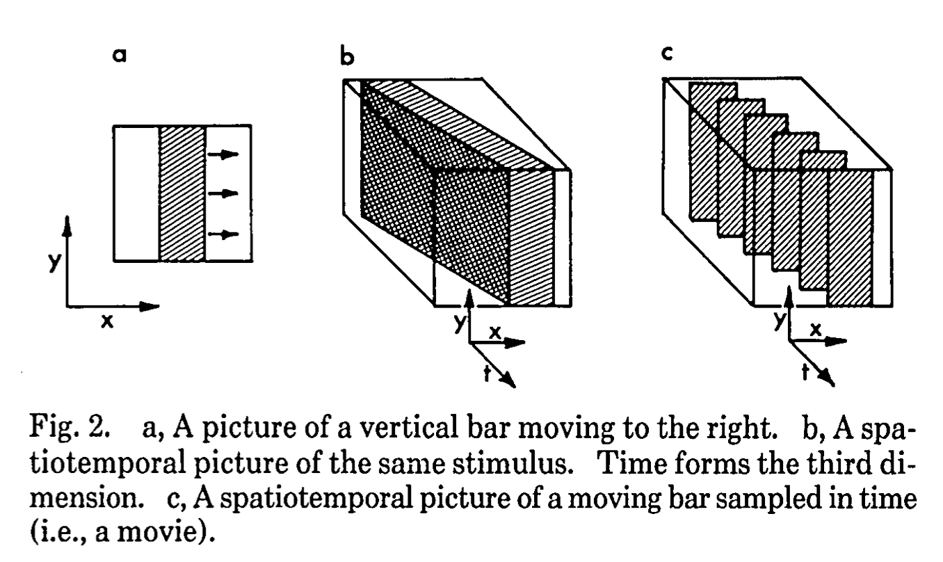
$x - y - t$ paths. We can think of particles as taking a path through $x - y - t$ space (3D space). This is a really interesting geometric way of thinking about motion. I think it might also be possible to add a natural extension of depth $z$ , at which point we have standard “spacetime”. A lot of the figures in the paper explore one-dimensional visual stimuli, and $x - t$ space is two-dimensional and thus very easily visualizable.

Sampling. All image/video signals are sampled; see the figure above (Fig 2). However, with some spatiotemporal blurring we can reconstruct the original signal: 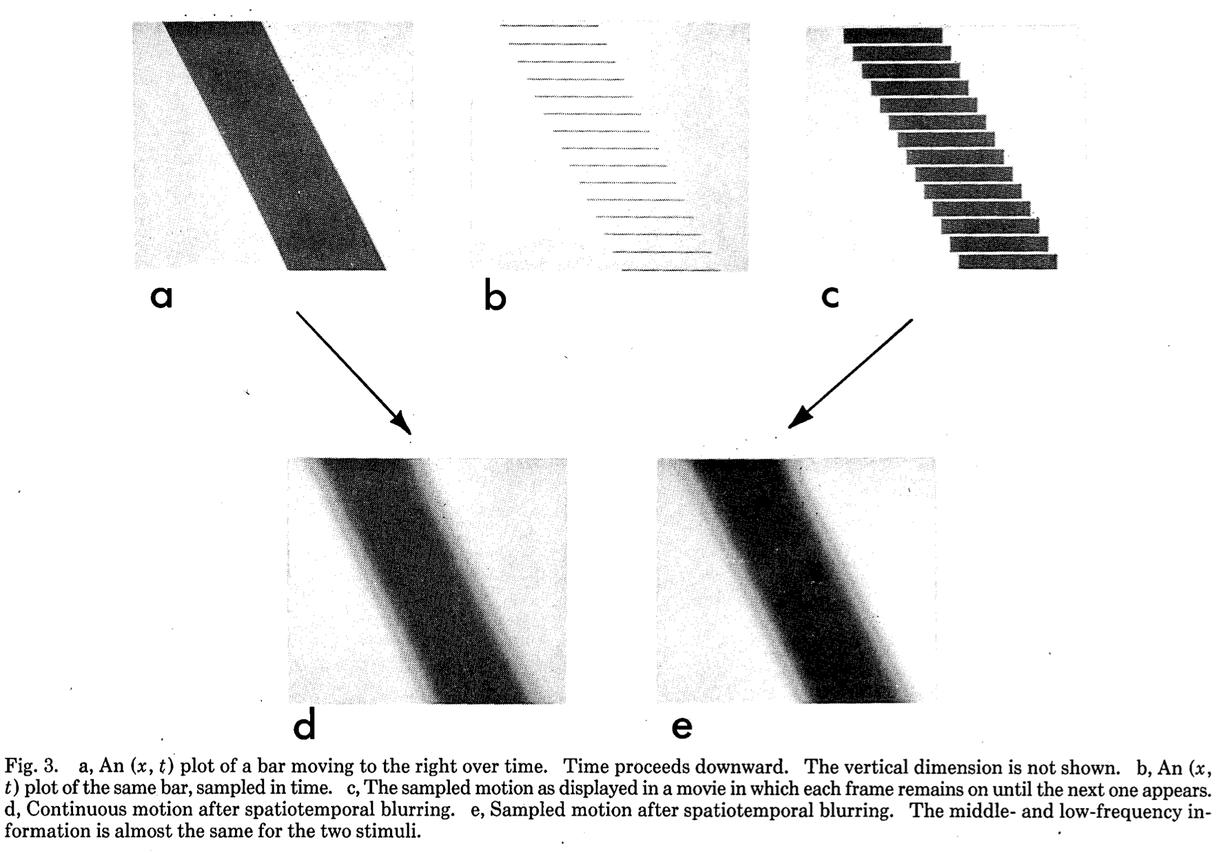Spatial blurring seems pretty common but I’m really curious what “temporal blurring” might look like. Taking simply the average of two frames doesn’t seem to make that much sense, especially with large motions; I think spatial blurring then followed by temporal blurring is the only thing that might make sense. When we advance to video, introducing temporal blurring might give us another axis of controllable “coarseness”.

Optical illusions. There’s a bit more context about this later on, but a really cool optical illusion is introduced in this paper, called reversed-phi. By inverting a moving image, the image’s motion can look continuous while nothing is really moving (that much). Here’s a website explaining it, and you can see an example here: This optical illusion gives a good example of the entanglement between our color vision and our motion processing, which makes sense given the filters explained below.

Hand-constructing an optical flow filter

A figure that summarizes the steps in hand-crafting optical flow.

Separable filters and a motion filter

First, we design a filter for general motion. In order to get a feel for what a filter like this may look like, we can:

envision stimuli as creating a path through $x - t$ space, like this:
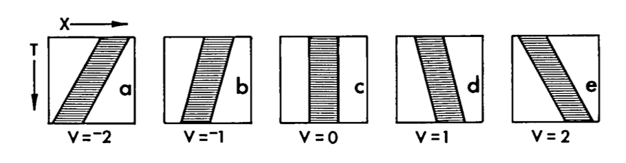
then convolutional filters can be envision as a weighting in 2D space, much like normal convolution filters, $R^{2} \to R$ . Then filters that look vaguely like this will be able to detect motion:

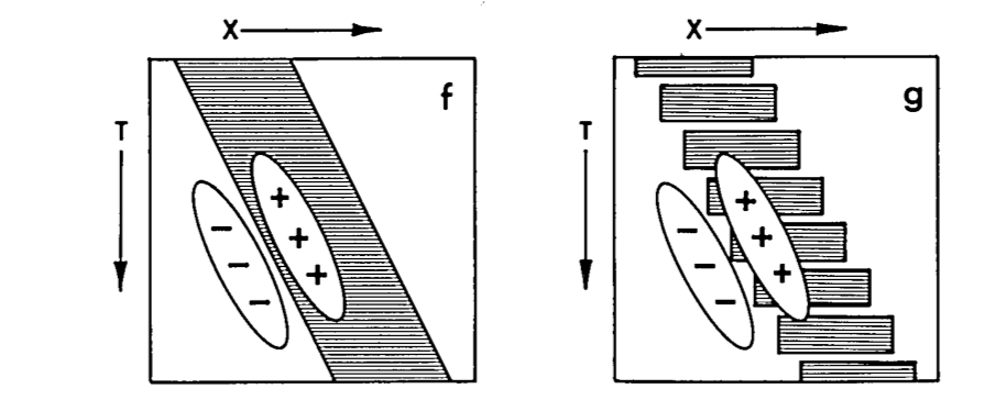
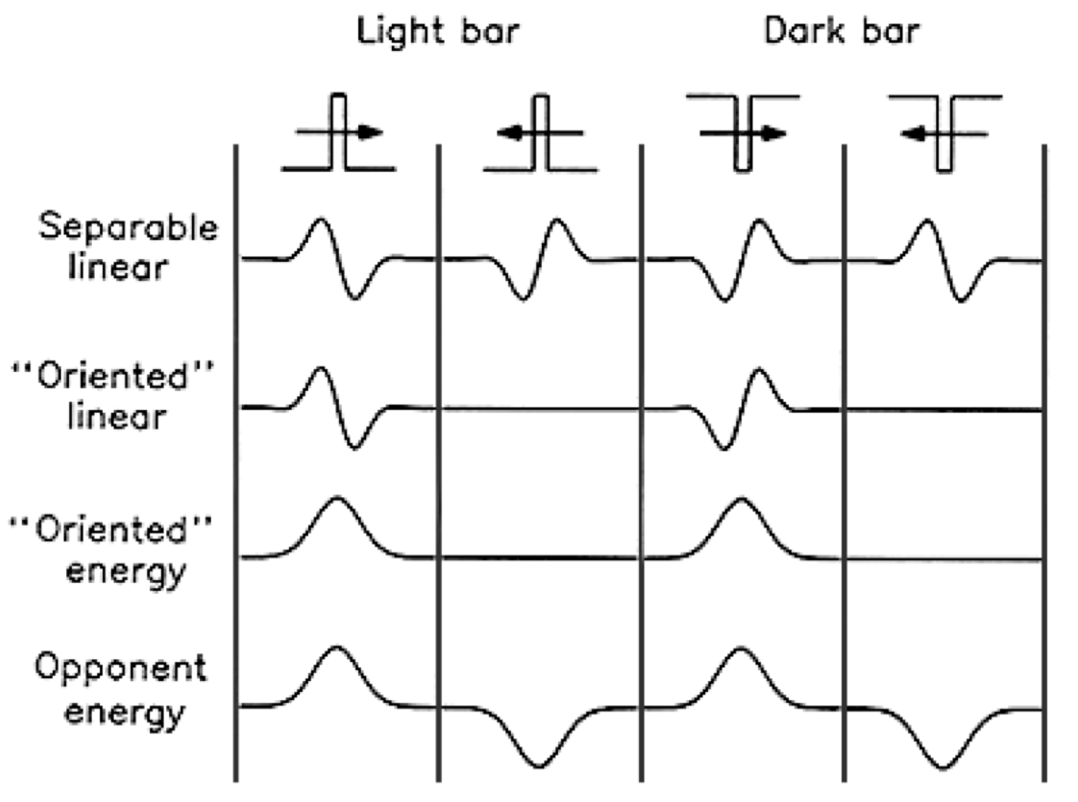
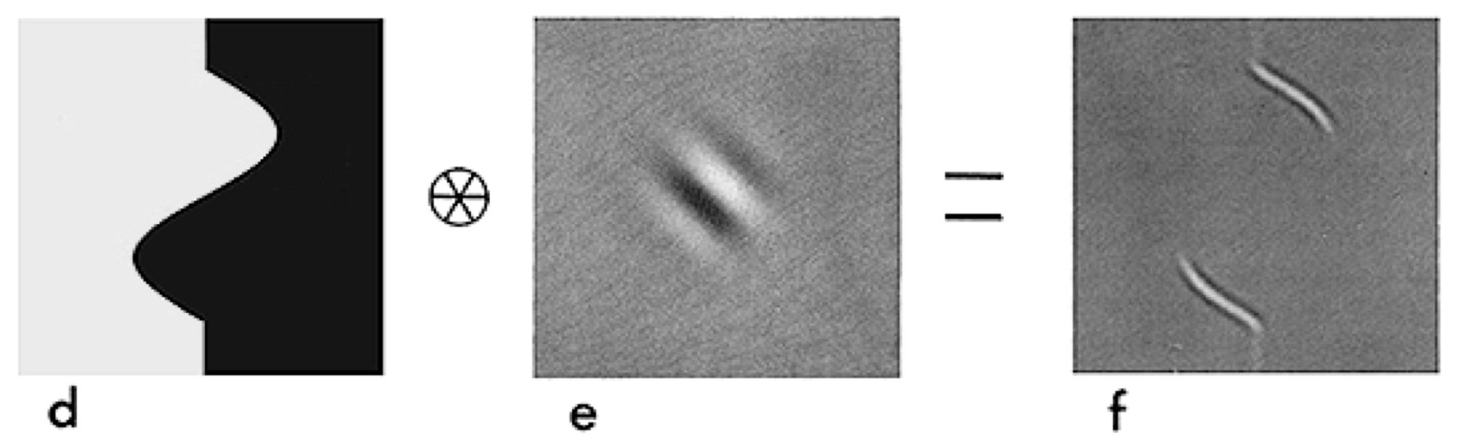
Indeed, we can construct a filter that looks pretty much like that. It will light up (either positive or negative, depending on direction & color) at any motion edges. For example, convolving a sinusoidal motion with an oriented Gabor function causes right motions to be detected:

Solving the phase problem

The problem with the above filter is that it is highly sensitive to whether or not the motion is “in-phase” with it, temporally or spatially. If it is out of phase, it may not detect motion at all. On the other hand, if it is in phase, it is sensitive to exactly what direction the contrast is (black on white vs. white on black, for instance), which seems quite undesirable! (Phase is what’s causing those black borders on the white lines above.)

In order to solve this, two filters which are $9 0^{\circ}$ out of phase can be used. As $sin^{2} x + cos^{2} x = 1$ , and the filters used above are based on sinuisoids, this ensures a constant response to the stimulus. 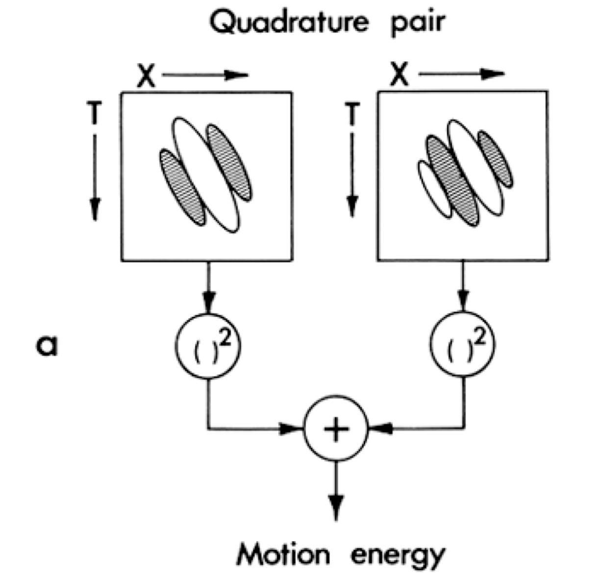They call this quantity “motion energy”, or “energy” for short. I think this is pretty different from the normal definition of energy in machine learning, i.e. it is actually the motion we are experiencing (optical flow), but it does share some similarities (always positive). I wonder if this sort of motivates some sort of multiplicative mechanism (attention maybe?) in our optical flow method.

Decomposition into separable filters

Separable filters are those decomposable as $f (x, t) = a (x) \cdot b (t)$ . Visually, they contain only horizontal and vertical lines; for example: 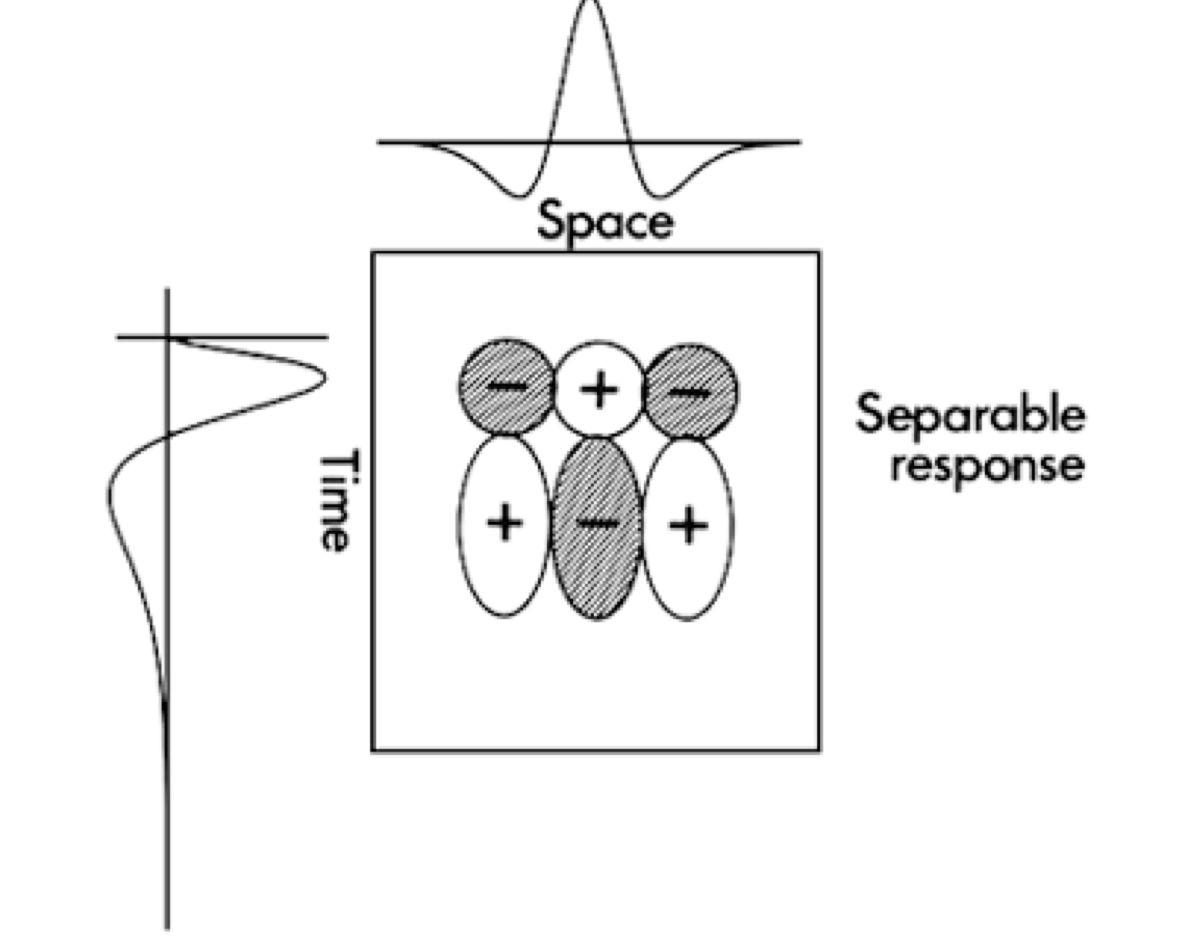I think the filters implemented inside the UNet right now are all separable actually, as they treat time as a channel and $x, y$ as space, so they have to be mutated independently of each other. Separable filters are believed by the authors to be more biologically plausible as well.

Separable filters can’t be sensitive to the direction of motion (makes sense as there can’t be any sloped boundaries). In order to reproduce the above filters with separable filters, we need to use many separable filters and add them up, e.g.:

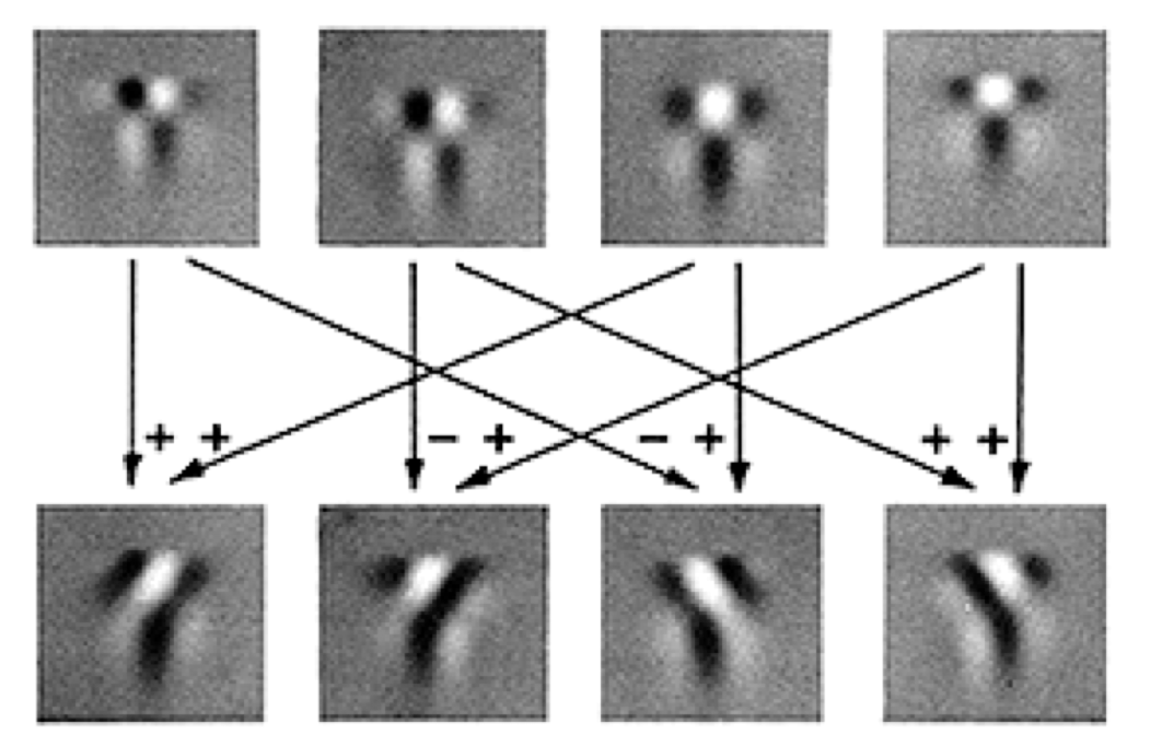
Going through all this pain simply to mimic other types of filters makes me think that a 3D UNet, which somehow innately allows all spatiotemporal filters, may be a better architecture than the current hacked 2D UNet.

From energy to velocity

In order to truly implement optical flow, we need the final output to be sensitive to the direction to motion (i.e. positive in one direction, zero if no motion, and negative in the other direction). This last step is pretty simple; they call it opponent energy. Pretty much just recreate the filters for the opposite direction and subtract one from the other; then you get a beautiful optical-flow like response.

Cited

None

Cited By

Return: index

Research

Table of Contents

1985.A&B—Spatiotemporal energy models for the perception of motion (Adelson & Bergen, 1985)

Some motivational ideas