1989.Fwork—A Computational Framework and an Algorithm for the Measurement of Visual Motion

Link to paper

A quite comprehensive reworking of methods for optical flow. They use the typical combination of elements (coarse-to-fine, photometric, and smoothness), but use two main strategies not present in other papers:

1. Explicit search for matching pixels. That is, they search over a narrow (3x3) grid around the current estimate at each level, in order to find the pixel with the most similar 5x5 neighborhood. The result is then smoothed with the smoothing loss.
2. A second-order confidence measure to weight different points and in particular different directions for the photometric loss (not the smoothness loss). They combine these with the three components mentioned above and then use an iterative method (much like Gauss-Seidel, etc.) in order to solve for $u$ and $v$.

Pyramid search advancements §

Bandpass filter. While constructing mid-levels, they first apply a low-pass filter (e.g. Gaussian blur) and then subtract frequencies below, leading to a band-pass filter. At each level, only a (narrow) range of frequencies are present in the image. This leads to less interference from other frequencies.

Overlapped pyramid. In a coarse-to-fine scheme, any mistakes at higher levels are propagated downwards:

The displacement at a pixel at a level $l-1$ is projected to the four pixels below at level $l$. However, in this scheme, if the displacement computed for a coarse-level pixel is incorrect, the search areas of none of its descendants at any of the subsequent levels will contain its correct match. Hence, a single match error made at a coarse level causes a large block of pixels at the image resolution to have incorrect displacements.

In order to fix this, they propose the following scheme: each pixel at level $l-1$ sends its prediction to a $4\times 4$ (versus $2\times 2$) grid below it. This gives each pixel at level $l$ 4 different match candidates to begin with: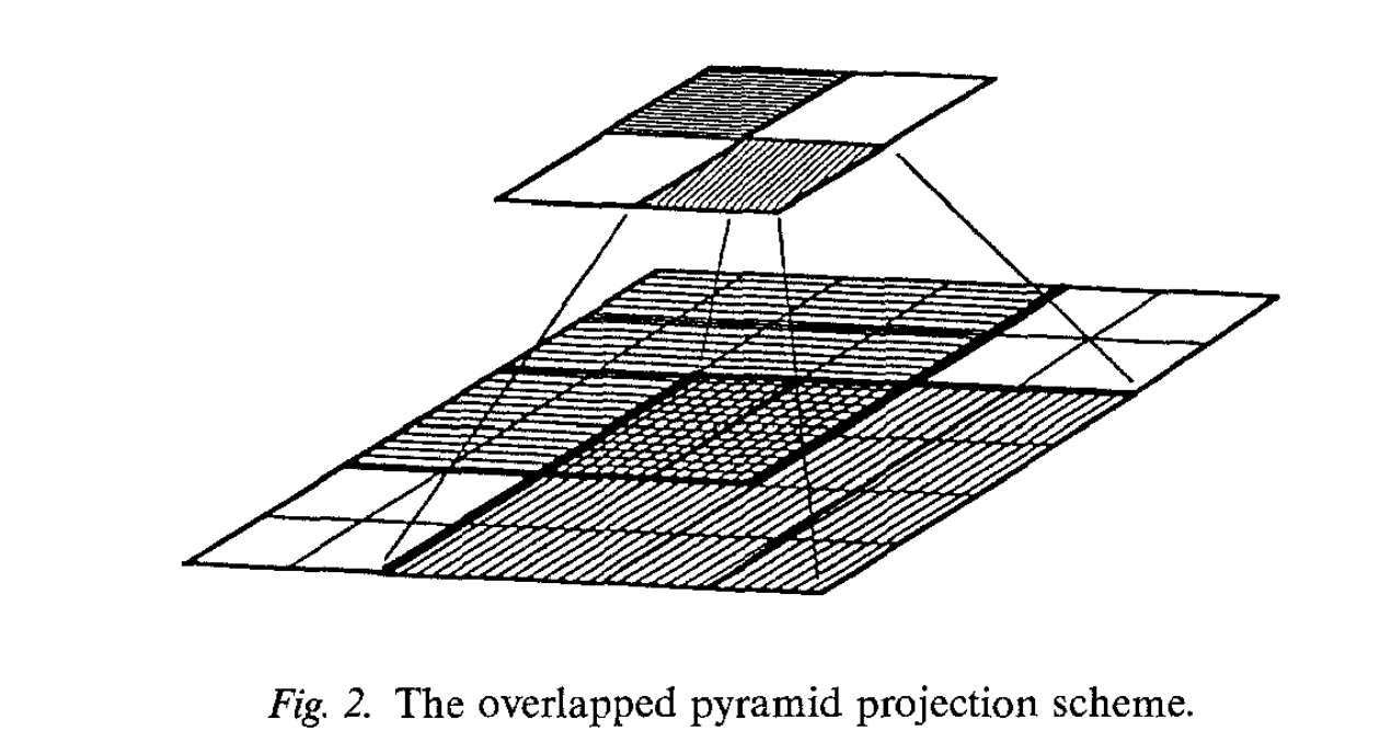

Matching based on context. Matches are not only done based on the pixel itself, but a 5x5 window around the pixel. I think this is related to gradient matching methods, as gradients are usually calculated with nearby pixels.

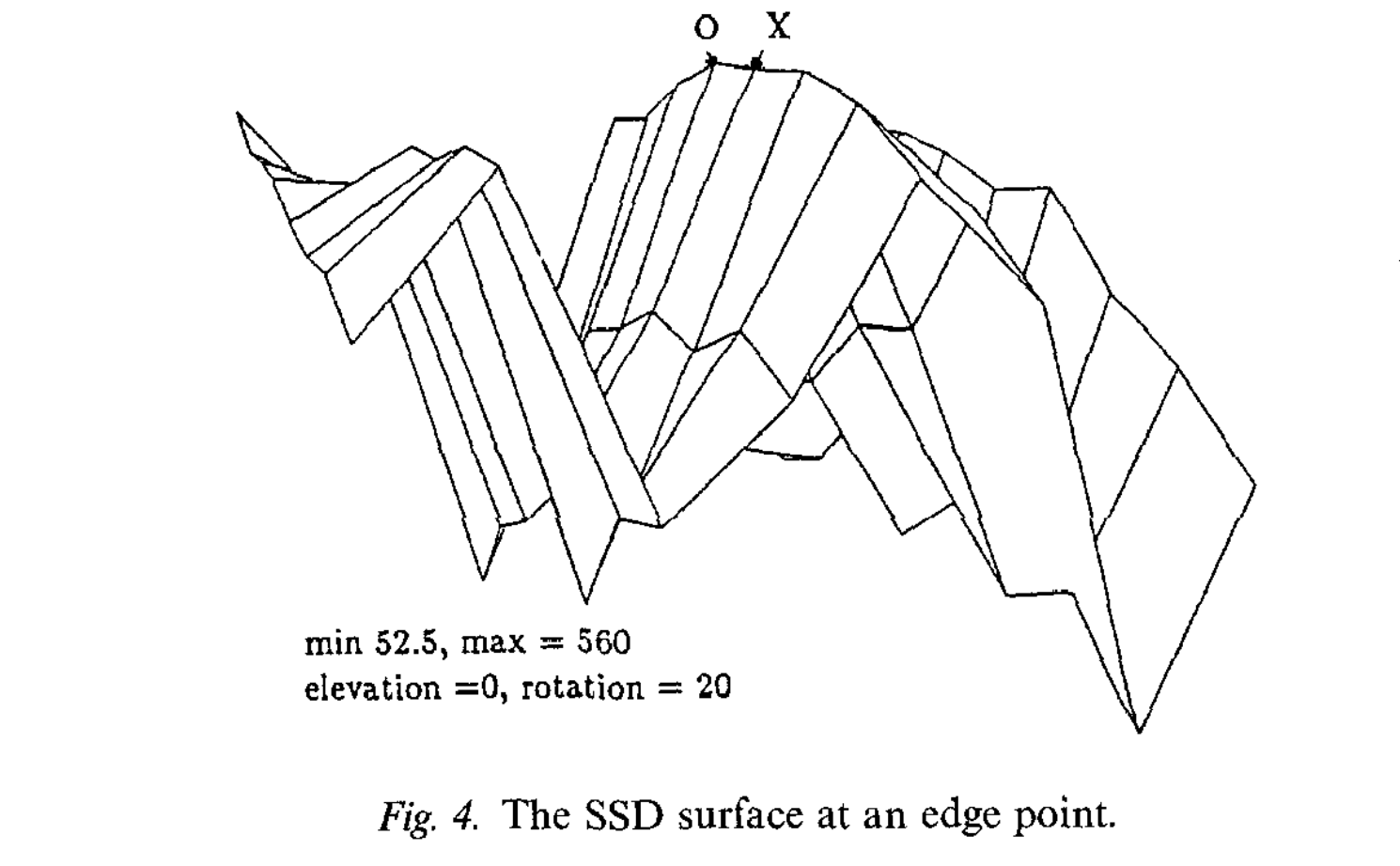
Some really cool visualizations §

I thought these figures were really interesting, to give an idea of what the loss landscape might look like: ![[Asset 5@2x.png]] The occlusion part always really confuses me though. Occluded pixels and disoccluded pixels should both have really high SSDs right? I guess that’s what the last figure shows, but it’s still a bit confusing.

Here’s another one, showing the nature of the aperture problem. The first one is with smoothing; the second one is without. It settles on the correct edge but not the correct location within that edge as it’s not well-specified. ![[Asset 1@2x.png]]

Adding smoothness to explicit search §

Adding in a smoothness condition makes a big difference in the final results: ![[Smoothing@2x.png]]

The way they do this is by using the pixel-matching SSD loss as a “ground-truth” optical flow, and the photometric loss measures the difference between the matched flow and the smoothed flow.

The “base” energy to be minimized is:

$$E(\{\mathbf{u}\})=E_{\text{sm}}(\{\mathbf{u}\})+E_{\text{ap}}(\{\mathbf{u}\})=\iint \text{trace}(\nabla {\mathbf{u}}^T{)}^T(\nabla {\mathbf{u}}^T)dxdy+\sum _{x,y}[(u_x-d_x{)}^2+(u_y-d_y{)}^2].$$

The first term is equivalent to the smoothness loss from H&S. The second would measure deviation from the match predictions $d_x$ and $d_y$, basically the same loss one would use for a GT optical flow in a supervised setting.

Confidence measure §

They propose an additional refinement, weighting the photometric loss by not only overall confidence but confidence in a particular direction. They use the second derivative (curvature) as a measure of confidence, letting ${\hat{\mathbf{e}}}_{max}$ and ${\hat{\mathbf{e}}}_{min}$ be the unit vectors in the directions of the greatest and least curvature, respectively, (I assume ${\hat{\mathbf{e}}}_{max}\perp {\hat{\mathbf{e}}}_{min}$) and then the above $E_{\text{ap}}(\{\mathbf{u}\})$ is replaced with

$$\sum _{x,y}{c}_{\text{max}}(\mathbf{u}\cdot {\hat{\mathbf{e}}}_{\text{max}}-\mathbf{d}\cdot {\hat{\mathbf{e}}}_{\text{max}}{)}^2+c_{\text{min}}(\mathbf{u}\cdot {\hat{\mathbf{e}}}_{\text{min}}-\mathbf{d}\cdot {\hat{\mathbf{e}}}_{\text{min}}{)}^2{c}_i=\frac{{\text{curvature}}_i}{k_1+k_2\cdot \text{min}(\text{SSD vals})}.$$

I’m not sure why they choose curvature (I guess it’s deviations from a linear local estimate?) as opposed to just the derivative itself. As opposed to N&E, the weightings are applied to the photometric loss, not the smoothness loss.

Iterative solution §

They use something called the finite element method to solve the minimization problem of $E$ above. I’m not really sure exactly how it’s involved here (in particular, what they describe seems pretty different from what I found online about it), but they end up with iterative update rule

$${\mathbf{u}}^{n+1}={\bar{\mathbf{u}}}^n+\frac{c_{\text{max}}}{c_{\text{max}}+1}((\mathbf{d}-{\bar{\mathbf{u}}}^n)\cdot {\hat{\mathbf{e}}}_{\text{max}}){\hat{\mathbf{e}}}_{\text{max}}+\frac{c_{\text{min}}}{c_{\text{min}}+1}((\mathbf{d}-{\bar{\mathbf{u}}}^n)\cdot {\hat{\mathbf{e}}}_{\text{min}}){\hat{\mathbf{e}}}_{\text{min}},$$

which converges towards the minimizer. They have a really cool diagram (I love the diagrams in this paper) intuitively showing what happens with each update of $\mathbf{u}$:

![[Screen Shot 2023-09-05 at 22.45.34.png|center|300]] ![[Screen Shot 2023-09-05 at 22.47.05.png|center|300]]

Tags §

Finite element method Energy or loss minimization Explicit search, matching Bandpass filters Multi-scale pyramids, coarse-to-fine NOT deep learning Old school Optical flowSmoothness constraints Unsupervised Upscaling flow

Cited §

• 1981.H&S—Determining Optical Flow (Horn & Schunck, 1981)
• 1981.L&K—An Iterative Image Registration Technique with an Application to Stereo Vision (Lucas & Kanade, 1981)
• 1985.A&B—Spatiotemporal energy models for the perception of motion (Adelson & Bergen, 1985)
• 1986.N&E—An Investigation of Smoothness Constraints for the Estimation of Displacement Vector Fields from Image Sequences (Nagel & Enkelmann, 1986)

Cited By §

• 2004.BBPW—High Accuracy Optical Flow Estimation Based on a Theory for Warping (Brox… 2004)

Return: index