2004.BBPW—High Accuracy Optical Flow Estimation Based on a Theory for Warping (Brox... 2004)

Link to paper

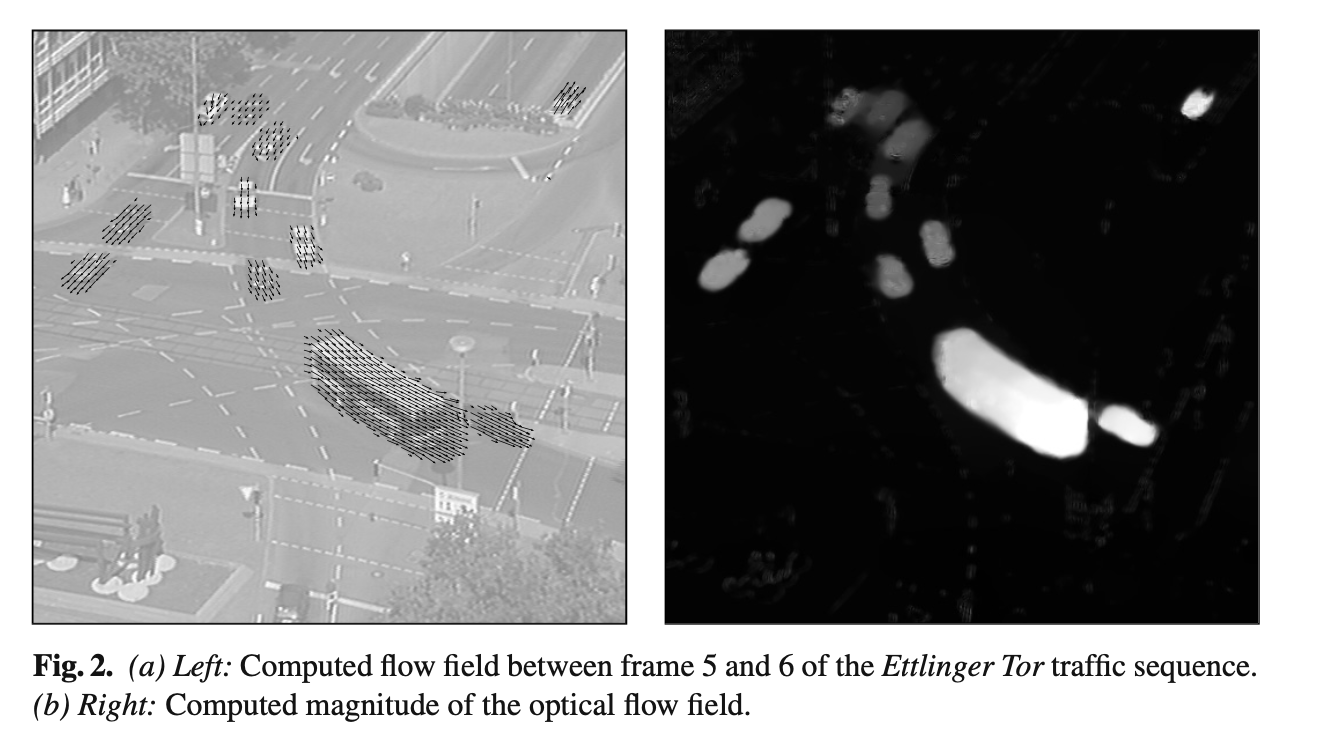
A classic old-school CV paper where optical flow is manually calculated & iterated upon for sequences of images (video). Like the classic approach, optical flow is formulated as satisfying constancy assumptions (color of a pixel does not change) and smoothness constraints (flow should be piecewise smooth). They use the variational method, i.e. modeling optical flow as a function.

Tags §

NOT deep learning Calculus of variations Unsupervised Optical flow Multi-scale pyramids, coarse-to-fine Energy or loss minimization Gradient constancy Smoothness constraints

Advancements in the energy function §

These all seem cool, but unfortunately ablation studies weren’t a thing in 2004, so I have no idea how each of them actually contributes to better performance.

De-linearization §

Let $I(x,y,t)$ be the pixel values of the image. The first improvement they do compared to H&S is to remove the implicit linearization in the brightness constancy (which they call grey-value constancy) equation:

$$I_{x}u+I_{y}v+I_t=0⟹I(x,y,t)=I(x+u,y+v,t+1).$$

While the first constraint involves partial derivatives and thus assumes the image changes linearly, flow displacements may be sufficiently large (and the images sufficiently quantized) that this is not the case. The latter constraint is now nonlinear due to the application of $I$, but more suitable for large displacements. However, it admits the existence of many local minima (which is why optical flow is hard).

Gradient constancy §

It was impossible for methods like H&S to deal with changes in shading. In order to be able to handle shading, we can also formulate the gradient constancy constraint, which is similar to the grey-value constancy constraint but only applies to the gradient of the image. Let $\nabla =({\partial }_x,{\partial }_y{)}^T$; then this constraint can be formulated as

$$\nabla I(x,y,t)=\nabla I(x+u,y+v,t+1),$$

and later on they set $\mathbf{w}=(u,v,1{)}^T$ for easier notation. Since the gradient is not modified by global brightness changes, this assumption is a bit more adaptable.

On the benefits of this assumption in particular, they write

The [gradient constancy] constraint is particularly helpful for translatory motion, while [the linear grey-value constancy] constraint can be better suited for more complicated motion patterns.

Note that F&W Optical Flow Overview discusses similar gradient constancy assumptions, so it seems like that this assumption is not really new to this paper. Additionally, there are downsides; patterns that are rotating or sheared will be penalized under the gradient constancy assumption.

The approach §

Energy formulation §

The photometric loss is

$$E_{Data}(u,v)={\int }_{\Omega }\Psi (|I(\mathbf{x}+\mathbf{w})-I(\mathbf{x}){|}^2+\gamma \cdot |\nabla I(\mathbf{x}+\mathbf{w})-\nabla I(\mathbf{x}){|}^2)d\mathbf{x}$$

and the smoothness loss is

$$E_{Smooth}(u,v)={\int }_{\Omega }\Psi (|\nabla u{|}^2+|\nabla v{|}^2)d\mathbf{x},$$

where $\Psi (x)=\sqrt{x^2+{\epsilon }^2}$ is the Charbonnier penalty and the second gradients are respect to $x,y,t$ respectively. As usual, the whole energy functional is equal to a weighted sum of these two terms: Apparently the smoothness loss allows piecewise smoothness, and is also a “total variation” loss, but I don’t understand why it incentivizes piecewise smoothness (as opposed to general smoothness).

Minimizing the energy §

This step involves a lot of math. Essentially, the Euler-Lagrange equation from the calculus of variations states that a minimizer $E(u,v)$ of the energy functional satisfies 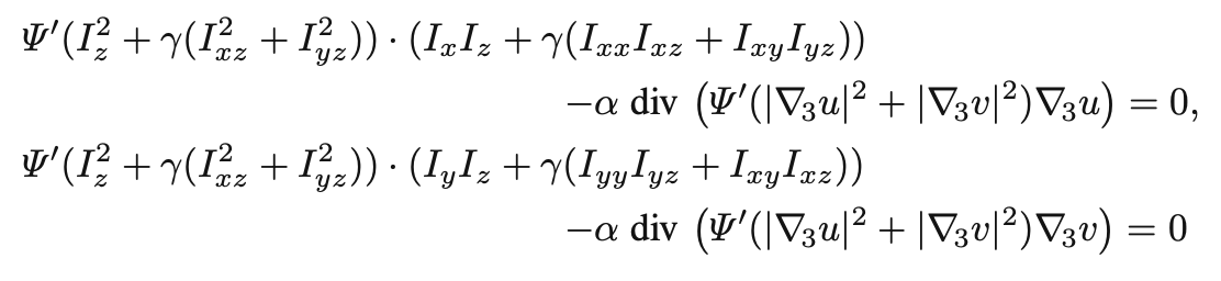The first equation corresponds to $u$ and the second to $v$; the first half of each equation corresponds to the $E_{Data}$ term and the second to the $E_{Smooth}$ term. The minimization process is iterative; I’ll describe it later. The $I_{\ast }$ terms denote different approximations of partial derivatives (i.e. $I_z=I(x+w)-I(x)$.)

Coarse-to-fine process Minimization is done in a multi-scale way. Scaling involves scaling down $I(x,y,t)$ by a factor $\eta \in (0,1)$ among the $x$ and $y$ dimensions. First, minimization is done over the lowest scale. Once it’s converged, the flow is upscaled(? actually it’s not super clear) to use as initialization for the next scale.

Big picture The equations need to be linearized in order to be solved with normal numerical methods. Thus we do something similar to EM:

1. Set ${\mathbf{w}}_0=(0,0,1{)}^T$.
2. Replace most (but not all) of the $\mathbf{w}$s with ${\mathbf{w}}_k$s, then the rest with ${\mathbf{w}}_{k+1}$ such that it’s linear in ${\mathbf{w}}_{k+1}$ (or in this case $(d{u}^{k+1},d{v}^{k+1},0)={\mathbf{w}}^{k+1}-{\mathbf{w}}^k$).
3. Solve for $d{u}^{k+1},d{v}^{k+1}$ (with an inner iteration), and add them back to $u,v$ to get ${\mathbf{w}}^{k+1}$.
4. Rinse and repeat with $k\leftarrow k+1$. The idea is that ${\mathbf{w}}^i$ will converge to a fixed point $\mathbf{w}$. This is called “fixed point iteration”; when a fixed point is reached, it solves the original equation. When we get something that solves the original equation, it is (probably) a minimizer of $E(x,y,t)$.

Nowadays, I think we’d just use a neural network to minimize that objective. Would it be better at it? Probably? It’s kind of shocking to me how this is basically the modern method for unsupervised optical flow, except we have neural nets instead of shitty equation solvers.

Theory of warping §

The authors promise a theory of warping, i.e. that warping is theoretically optimal. One of their comments is exactly what I’ve been thinking about for a while:

Thus, the estimated used to have a magnitude of less than one pixel per frame, independent of the magnitude of the total displacement.

I don’t really get the theory; I’m going to read the reference [17] and maybe come back to it?

Cited §

• 1981.L&K—An Iterative Image Registration Technique with an Application to Stereo Vision (Lucas & Kanade, 1981)
• 1986.N&E—An Investigation of Smoothness Constraints for the Estimation of Displacement Vector Fields from Image Sequences (Nagel & Enkelmann, 1986)
• 1989.Fwork—A Computational Framework and an Algorithm for the Measurement of Visual Motion
• 1992.ROF—Nonlinear total variation based noise-removal algorithms
• 1996.B&A—The Robust Estimation of Multiple Motions. Parametric and Piecewise-Smooth Flow Fields (Black & Anandan, 1996)

Cited By §

• ! 2017.DSTFlow—Unsupervised Deep Learning for Optical Flow Estimation (Ren… 2017)

Return: index