1986.N&E—An Investigation of Smoothness Constraints for the Estimation of Displacement Vector Fields from Image Sequences (Nagel & Enkelmann, 1986)

Link to paper

Modifications to H&S are proposed to improve performance. The most discussed one is an edge/curvature aware smoothness constraint, i.e. a matrix with weights $\mathbf{W}$ such that we can modify the Horn & Schunck energy to

$$\int \int (g_2(\mathbf{x})-g_1(\mathbf{x}-\mathbf{u}){)}^2+{\alpha }^2\cdot \text{trace}((\nabla \mathbf{u}{)}^T\mathbf{W}(\nabla \mathbf{u}))dxdy,$$

noting that the $\mathbf{u}$ here is a backward flow, $\nabla \mathbf{u}$ is a matrix of partial derivatives:

$$\nabla \mathbf{u}=\left(\begin{array}{cc}{u}_x& v_x\\ u_y& v_y\end{array}\right),$$

$g_2,g_1$ are the images, and ${\alpha }^2$ is the weight of the smoothness loss. H&S is a special case of this where $\mathbf{C}=\mathbf{I}$. The proposed $\mathbf{W}$ is approximately[^1: there is a slight change; see the last point of ‘other advancements’] the symmetric

$$\mathbf{W}=\left(\begin{array}{c}{g}_y\\ -g_x\end{array}\right){\left(\begin{array}{c}{g}_y\\ -g_x\end{array}\right)}^T+b^2\cdot \left(\begin{array}{cc}{g}_{yy}& -g_{xy}\\ -g_{xy}& g_{xx}\end{array}\right){\left(\begin{array}{cc}{g}_{yy}& -g_{xy}\\ -g_{xy}& g_{xx}\end{array}\right)}^T,$$

where $b^2$ is a weighting parameter (discussed below). Note the presence of second order/curvature constraints as opposed to merely first-order constraints in typical edge-aware smoothness. The parameters used are ${\alpha }^2=1,c=8,\gamma =12.5$ (all discussed below).

A variety of other advancements are discussed as well. I think these will be useful for our method too in order to improve performance.

Tags §

Smoothness constraints Energy or loss minimization NOT deep learning Old school Unsupervised Optical flow Unsupervised Second-order methods

Other advancements §

1. Delinearization. Delinearization, discussed by the derivative work BBPW, wherein the linearized constraint $g_{x}u+g_{y}v+g_t=0$ is replaced with the delinearized version $g_2(\mathbf{x})-g_1(\mathbf{x}-\mathbf{u})=0$. This, on its own, leads to a huge performance gain.
2. Corners computed first. Corners with significant gray value variation are first computed, as their movement can be easily tracked, with the other areas are initially left blank. If $\kappa ,\lambda$ are the eigenvalues of $\mathbf{C}$, corners are when $\kappa \approx \lambda$ (and, I assume, $\det \mathbf{C}\gg 0$), as $\mathbf{C}$ contains values about the first- or second-derivatives at that point. The metric used to determine “cornerness” is $1\ge \frac{\det \mathbf{C}}{{\left(\frac{1}{2}\text{trace}\mathbf{C}\right)}^2}=\frac{4\kappa \lambda }{(\kappa +\lambda {)}^2}>\text{threshold}.$During this computation, the smoothness weight ${\alpha }^2$ is set to $0$. Then, after this computation is complete, the edge flows are propagated inwards and ${\alpha }^2$ is set upwards again.
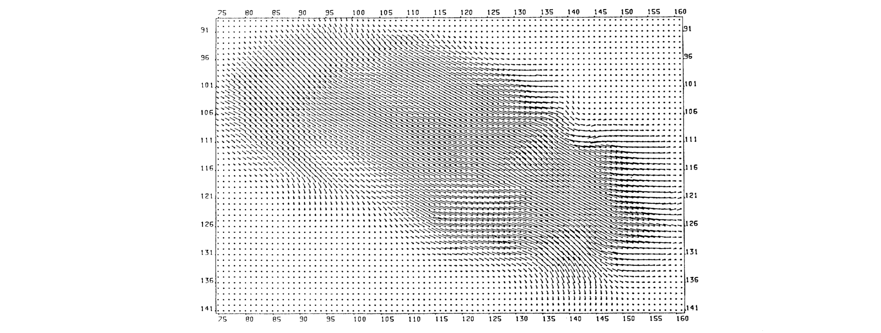
3. Smoothness scheduling. A schedule for the smoothness parameter ${\alpha }^2$ which looks like this:![[Screen Shot 2023-08-31 at 20.13.21.png|center|450]]
4. Temporal averaging for gradients. Improving gradients with temporal averaging, i.e. replace $g_1(\mathbf{x}-{\mathbf{u}}_0{)}_x$ with $\frac{g_2(\mathbf{x}{)}_x+g_1(\mathbf{x}-{\mathbf{u}}_0{)}_x}{2}$ (where ${\mathbf{u}}_0$ is the current estimate for $\mathbf{u}$).
5. Setting a lower limit $\gamma =2{\sigma }^2$ (5-12) for the eigenvalues of $\mathbf{C}$, above which the eigenvalues are rounded up.
6. Some small thing about Beaudet’s operator which I think is related in spirit to my problem of needing GT flow to be precisely 0. I don’t really get it and I don’t think it’s super relevant.
7. Something I get even less about adding something to the diagonal elements of $\mathbf{C}$.

Intuition for the weights ${\mathbf{C}}^{-1}$ §

Scaling effect of a weight matrix §

From H&S, we have the smoothness term

$$u_x^2+u_y^2+v_x^2+v_y^2=\text{trace}[(\nabla \mathbf{u}{)}^T\nabla \mathbf{u}],\nabla \mathbf{u}=\left(\begin{array}{cc}{u}_x& v_x\\ u_y& v_y\end{array}\right).$$

But we don’t care about all $u_x$, etc. In directions with high visual contrast (gradients), we want to suppress the smoothness loss in favor of the photometric loss. Thus, if $\kappa$ and $\lambda$ are rough measures of the size of the gradients in the $x$ and $y$ directions, respectively, we have the nice property

$$\text{trace}\left[(\nabla \mathbf{u}{)}^T{\left(\begin{array}{cc}\kappa & 0\\ 0& \lambda \end{array}\right)}^{-1}(\nabla \mathbf{u})\right]=\frac{u_x^2}{\kappa }+\frac{u_y^2}{\lambda }+\frac{v_x^2}{\kappa }+\frac{v_y^2}{\lambda }.$$

Finding $\mathbf{C}$ §

We derive $\mathbf{C}$ itself through another method. First, we begin with two heuristics.

1. $\nabla \mathbf{u}$ should be close to $0$ along the directions within an object. One such direction is the tangent to the object’s boundary; thus $\nabla \mathbf{u}\cdot (\nabla \mathbf{g}{)}^{\perp }\to 0$. We can write the norm of that expression as $\left({\left(\begin{array}{c}{g}_y\\ -g_x\end{array}\right)}^T\nabla \mathbf{u}\right){\left({\left(\begin{array}{c}{g}_y\\ -g_x\end{array}\right)}^T\nabla \mathbf{u}\right)}^T=\text{trace}\left((\nabla \mathbf{u}{)}^T\left(\begin{array}{c}{g}_y\\ -g_x\end{array}\right){\left(\begin{array}{c}{g}_y\\ -g_x\end{array}\right)}^T(\nabla \mathbf{u})\right).$
2. We can use a second-order constraint similar to the one above. That is, $\nabla \mathbf{u}$ should be maximal in the direction of greatest curvature; thus it should be around zero in the direction perpendicular to that of greatest curvature. This leads us to minimize ${\left(\begin{array}{cc}{g}_{yy}& -g_{xy}\\ -g_{xy}& g_{xx}\end{array}\right)}^T(\nabla \mathbf{u})$ which leads to a similar metric $\text{trace}\left((\nabla \mathbf{u}{)}^T\left(\begin{array}{cc}{g}_{yy}& -g_{xy}\\ -g_{xy}& g_{xx}\end{array}\right){\left(\begin{array}{cc}{g}_{yy}& -g_{xy}\\ -g_{xy}& g_{xx}\end{array}\right)}^T(\nabla \mathbf{u})\right).$

This leads us to a weighting matrix $\mathbf{F}$ where $\mathbf{F}=\left(\begin{array}{c}{g}_y\\ -g_x\end{array}\right){\left(\begin{array}{c}{g}_y\\ -g_x\end{array}\right)}^T+b^2\cdot \left(\begin{array}{cc}{g}_{yy}& -g_{xy}\\ -g_{xy}& g_{xx}\end{array}\right){\left(\begin{array}{cc}{g}_{yy}& -g_{xy}\\ -g_{xy}& g_{xx}\end{array}\right)}^T,$and $b$ is some weighting parameter between these two objectives. However, we would like to normalize $\mathbf{F}$, as it might take on large values (especially being quadratic). Thus we divide by the determinant (recall that the derivative is the factor by which a matrix increases volume) to yield

$${\mathbf{C}}^{-1}=\frac{\mathbf{F}}{\det \mathbf{F}},$$

which yields $\mathbf{C}$ as above.

In connection with the argument above, note that the top-left entry in $\mathbf{C}$ is all various derivatives/partials over $x$, measuring variation in $x$, and the bottom-right entry in $\mathbf{C}$ is all various derivatives/partials over $y$.

Cited §

• Rotationally Invariant Image Operators, P.R. Beaudet—Can’t find the paper online
• 1981.H&S—Determining Optical Flow (Horn & Schunck, 1981)

Cited By §

• 2004.BBPW—High Accuracy Optical Flow Estimation Based on a Theory for Warping (Brox… 2004)

Return: index