1981.L&K—An Iterative Image Registration Technique with an Application to Stereo Vision (Lucas & Kanade, 1981)

Link to paper Link to wiki

The classic local method for computing optical flow. It’s actually not an optical flow paper; they tackle what is called the image registration problem. For example, if you have many exposures of the same image (e.g. in astrophotography), but each image is slightly offset due to noise, the different exposures need to be aligned before combining in order to create a sharp image.

In contrast to optical flow, one global distortion is expected as opposed for the entire image or region. This does make it suitable for optical flow problems where the flow is expected to be relatively constant in an area; applying L&K locally gets you an estimate of the optical flow at that point.

Key assumptions. Local methods like L&K work only in a narrow range of cases.

• Optical flow is relatively constant in the given region of the image. (This is roughly equivalent to the smoothness assumption from H&S.)
• Optical flow is relatively small (around less than $1$ pixel).
• We have no textureless interiors we care about, which would erroneously have $0$ optical flow. Unlike H&S, edge optical flows cannot be propagated inwards to the interior of an object. Additionally, L&K is typically used to get sparse flows. There is, to my knowledge, no guarantee of smoothness.[^1: There may be, but it’s not mentioned in the paper.]

By incorporating the visual content of many pixels into the estimate of a single optical flow vector, L&K can get more accurate & robust (to noise) estimations of individual flows. However, it is difficult to get dense estimations.

Tags §

Multi-scale pyramids, coarse-to-fine NOT deep learning Old school Optical flow Stereo vision Unsupervised Local methods Unsupervised Affine, parameterized optical flow

The approach §

We are given a picture of size $N$, i.e. with $N^2$ pixels. Naively, if the flow is restricted to $M$ in each direction, we can attempt to iterate over all $O(M^2)$ possibilities, yielding a search time of $O(M^2{N}^2)$. L&K propose a hill-climbing method (i.e. gradient-descent type method) which uses gradients of the image (or approximations, i.e. $\nabla I_x\approx I(x+1)-I(x)$) in order to estimate which step to take next. Thus, unless a coarse-to-fine approach is used, optical flows should be $<1$ pixel.

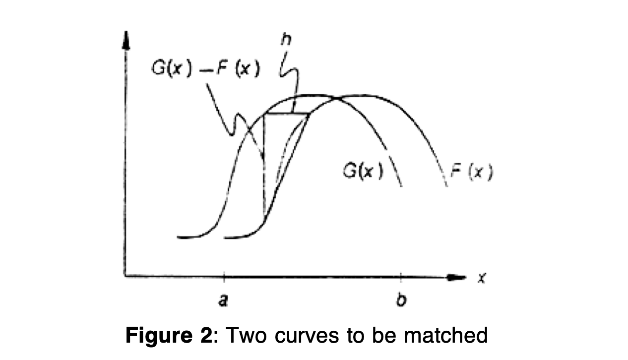
Given an image $F(x)$ and a second image $G(x)$, we wish to find a single vector $h$ which minimizes (primarily) the $L_2$ norm:

$${\left(\sum _{x\in R}[F(x+h)-G(x){]}^2\right)}^{1/2}.$$

We use an iterative method. In particular, let $h_0=0$ and $w(x)=\frac{1}{|G^{\prime }(x)-F^{\prime }(x)|}$, then

$$h_{k+1}=h_k+\sum _x\frac{w(x)[G(x)-F(x+h_k)]}{F^{\prime }(x+h_k)}\cdot {\left(\sum _{x}w(x)\right)}^{-1},$$

or (second variant)

$$h_{k+1}=h_k+\frac{{\sum }_{x}w(x)\cdot F^{\prime }(x+h_k)[G(x)-F(x+h_k)]}{{\sum }_{x}w(x)\cdot F^{\prime }(x+h_k{)}^2}.$$

The rough/intuitive derivation of these is as follows. Suppose we have the correct $h$. Then

$$F^{\prime }(x+h_0)=\frac{F(x+h)-F(x+h_0)}{h-h_0}=\frac{G(x)-F(x+h_0)}{h-h_0},$$

which implies $h-h_0=\frac{G(x)-F(x+h_0)}{F^{\prime }(x+h_0)}$ after rearranging. So then given an estimate $h_0$, we can estimate the error as such.

These two variations are just different weighting methods for different terms of that form. Note that a lot of linearizations are used in the derivation of these formulas.

Low frequency signals §

Here’s a really interesting passage from the paper: Smoothing via blurring kind of implicitly enables a coarse-to-fine approach. Thus I’m wondering if instead of using a pure pyramid loss, we could blur the image significantly instead to induce the same low-frequency gradients. Right after this, they propose using a coarse-to-fine strategy in order to speed up calculations.

Generalizations and applications §

First, they extend to multiple dimensions. The vectorized form of the second equation is:

$$h=\left[\sum _x{\left(\frac{\partial F}{\partial x}\right)}^T[G(x)-F(x)]\right]{\left[\sum _x{\left(\frac{\partial F}{\partial x}\right)}^T\left(\frac{\partial F}{\partial x}\right)\right]}^{-1}.$$

Then, they discuss a generalization of the above approach to a general affine transform $Ax+h$, where both $A$ and $h$ are optimized for. Interestingly, I think this would be super flexible with scaling of image objects, whereas most optical flow methods would struggle with this.

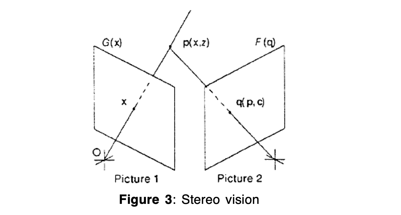Finally, they describe an application of this approach to stereo vision, where we want to estimate the relative poses of the two cameras as well as the depth of the image. The affine transform mentioned in the previous part is useful here; I didn’t read it very carefully.

Cited §

None

Cited By §

• 2004.BBPW—High Accuracy Optical Flow Estimation Based on a Theory for Warping (Brox… 2004)
• ! 2005.F&W—Optical Flow Estimation (Fleet & Weiss, 2005)

Return: index