1981.H&S—Determining Optical Flow (Horn & Schunck, 1981)

Link to paper Link to wiki

Super old-school, seminal paper on how to calculate optical flow. Primarily proposes the two constraints still mainly used today:

1. brightness constancy; that a pixel’s color/brightness doesn’t change over time (brightness in grayscale, RGB in color)
2. smoothness; that most derivatives (or second derivatives) of the flow should be zero. These constraints are directly optimized for, per-image-pair, with an iterative scheme. There’s also some math (calculus of variations???) that I don’t understand. Additionally, introduces standard notation of $u$ and $v$ as $dx/dt$ and $dy/dt$ of a particle/pixel.

Apparently this is a “global” method, as opposed to L&K which is a “local” method.

According to Ayush, H&S works really well; i.e. it was not beat by deep learning methods until around ~2015, which is a bit shocking.

Tags §

Old school NOT deep learning Unsupervised Optical flow Calculus of variations Energy or loss minimization

Laplacian weighting §

The weighting in order to approximate the Laplacian ${\left(\frac{dx}{dt}\right)}^2+{\left(\frac{dy}{dt}\right)}^2$ looks like this, with $1/6$ and $1/12$ at the neighboring cells:

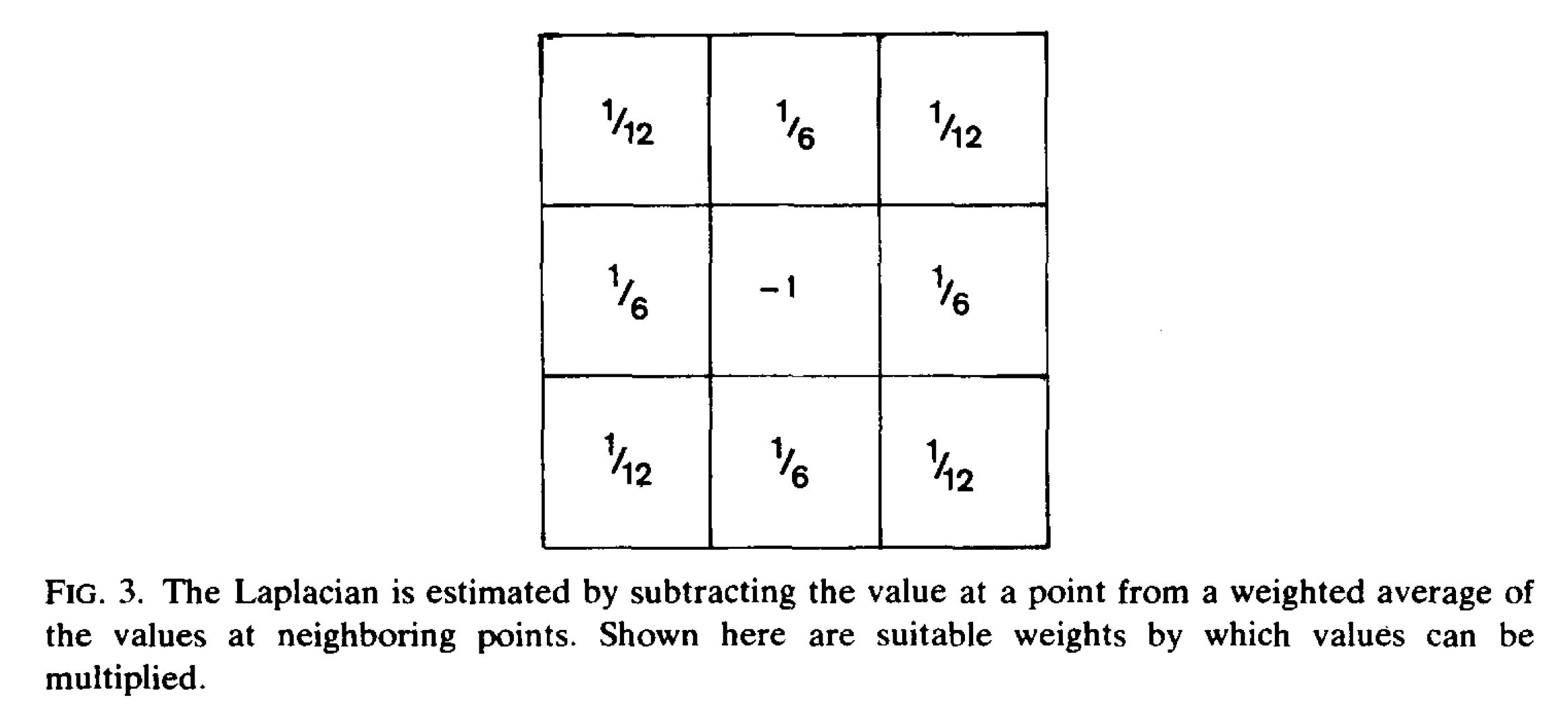
In simple situations, both Laplacians [of $u$ and $v$] are zero. If the viewer translates parallel to a flat object, rotates about a line perpendicular to the surface or travels orthogonally to the surface, then the second partial derivatives of both $u$ and $v$ vanish.

Formulation of the two constraints §

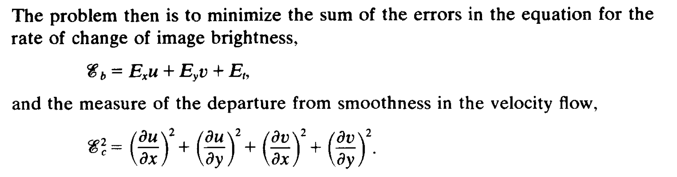These are minimized in the ratio $1:{\alpha }^2$. The first one gives an estimate of how much $dE/dt\ne 0$, i.e. brightness changes (it seems related to the classic photometric loss). However, as opposed to modern photometric losses, this seems to look really closely at the derivatives around a single point.

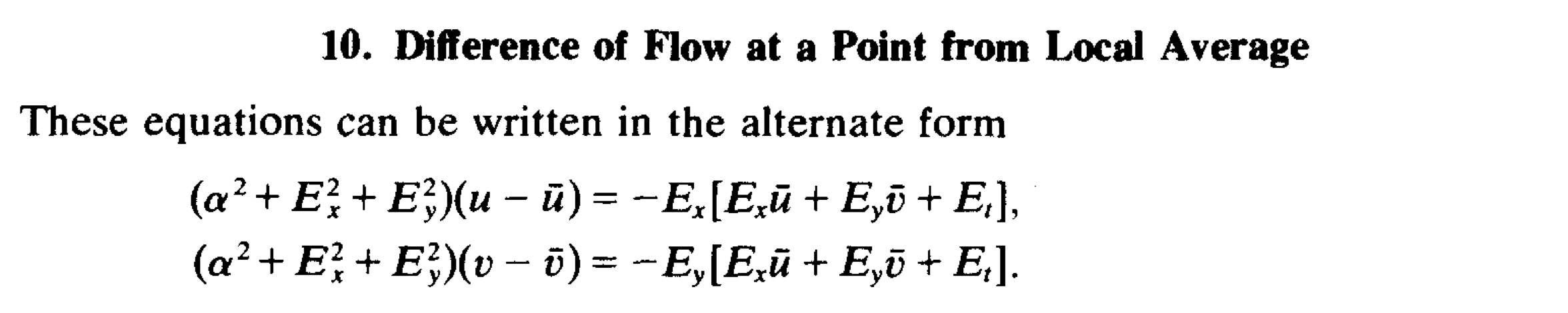
Ultimately, considering a noise level $\alpha$, the following pair of equations for each point is derived:

One thing I’m quite curious about is if using these constraints instead of modern constraints (which are a bit more simple) would lead to better performance. Question: are there any papers that try to use these constraints combined with modern deep learning?

Finally, in order to solve these equations, iteration is employed. $\bar{u}$ and $\bar{v}$ are taken from the previous iteration and then $u$ and $v$ are solved for directly. Eventually, a fixed point is converged upon, which solves the above equations. 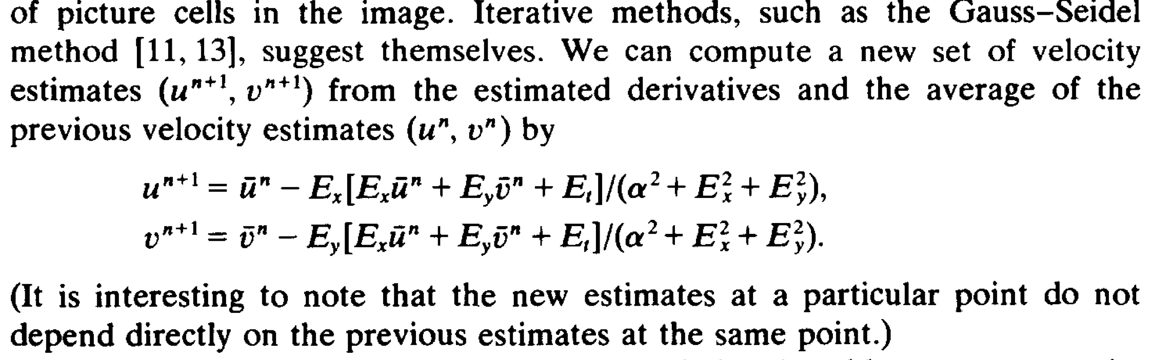Note that the second term seems normalized with respect to $E_x$, $E_y$ and seems to mostly depend on the ratios $E_x:E_y$ (as long as $\alpha$ is small).

Quotes §

There are a number of cute quotes that outlines things that are still true today, forty years later, which I find really interesting.

The previous state of optical flow estimation §

These papers begin by assuming that the optical flow has already been determined. Although some reference has been made to schemes for computing the flow from successive views of a scene, the specifics of a scheme for determining the flow from the image have not been described.

On why optical flow is difficult §

Optical flow cannot be computed locally, since only one independent measurement is available from the image sequence at a point, while the flow velocity has two components. A second constraint is needed.

Edge cases for optical flow §

Consider, for example, a patch of a pattern where brightness varies as a function of one image coordinate but not the other. Movement of the pattern in one direction alters the brightness at a particular point, but motion in the other direction yields no change.

We perceive motion when a changing picture is projected onto a stationary screen, for example.

Consider, for example, a uniform sphere which exhibits shading because its surface elements are oriented in many different directions. Yet, when it is rotated, the optical flow is zero at all points in the image, since the shading does not move with the surface.

Ignoring occlusions because they’re hard §

We exclude situations where objects occlude one another, in part, because discontinuities in reflectance are found at image boundaries…

An iterative solution §

The paper ends up using an iterative solution to solve the $2HW$ equations posed above. It seems like iteration is key to pretty much all optical flow(? or beyond) methods. There is also some choices one can make when it comes to the particular way iteration is performed:

As a practical matter one has a choice of how to interlace the iterations with the time steps. On the one hand, one could iterate until the solution has stabilized before advancing to the next image frame. On the other hand, given a good initial guess one may only need one iteration per time step. A good initial guess for the optical flow velocities is usually available from the previous time-step.

That last idea seems critical to the performance of RAFT, for instance. Up to around 64 iterations are performed.

Filling in uniform regions §

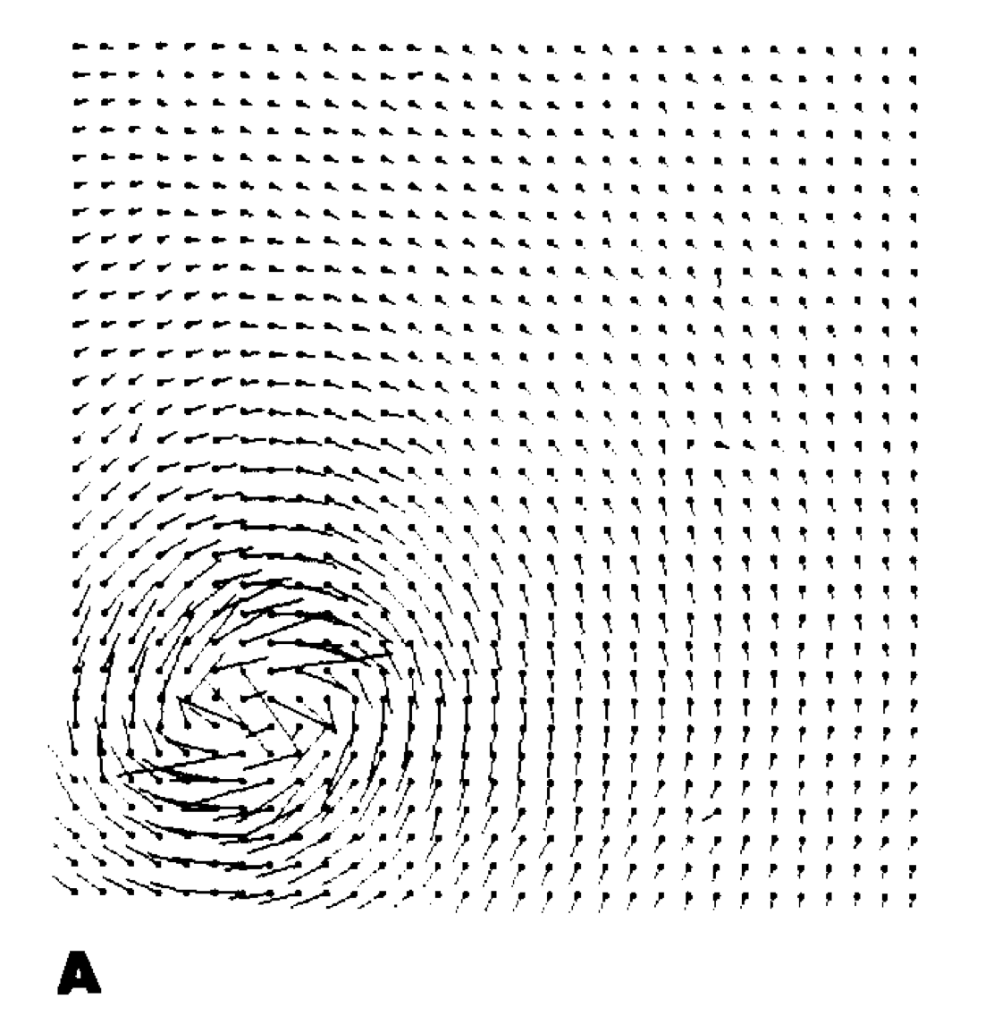
Much like I think any self-supervised optical flow method would, uniform/untextured regions are slowly filled in from the edges:

In parts of the image where the brightness gradient is zero, the velocity estimates will simply be averages of the neighboring velocity estimates… Eventually the values around such a [uniform] region will propagate inwards.

Cited §

None

Cited by §

• ! 2017.DSTFlow—Unsupervised Deep Learning for Optical Flow Estimation (Ren… 2017)
• 2004.BBPW—High Accuracy Optical Flow Estimation Based on a Theory for Warping (Brox… 2004)

Return: index